Checks of Anaqsim
To save any of the associated files, right-click on the file link and select “Save link as…”.
Check 1: Uniform flow in a confined aquifer.
Check 2: Uniform flow in a confined aquifer with uniform recharge.
Check 3: Uniform flow in a confined aquifer with uniform leakage from below.
Check 4: Uniform flow in an unconfined aquifer with uniform recharge.
Check 5: Uniform flow in a confined interface aquifer with uniform recharge.
Check 6: Uniform flow in an unconfined interface aquifer with uniform recharge.
Check 7: Uniform flow in an unconfined aquifer with uniform recharge and two levels.
Check 8: Uniform flow in a two-level confined aquifer system with a circular opening connecting the two levels, like example 31.1 on pages 369-370 of Strack (1989).
Check 9: Transient simulation of theTheis (1935) solution.
Checks confined domains, spatially-
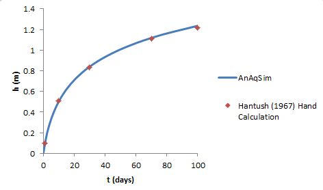
Check 10: Transient simulation of the Hantush (1967) analytic solution for mounding under a rectangular recharge area.
Checks unconfined domains, spatially-
Check 11: Comparison of complex multi-level Anaqsim model and equivalent MODFLOW 2005 model.
Checks confined, unconfined domains, transient and steady flow, spatially-
- Model description and plots comparing results of steady and transient models: CompareModels.pdf
- AnAqSim input files and the starting head file for the transient runs: AnAqSimFilesCheckMF.zip
- MODFLOW input files and ModelMuse input file that created the MODFLOW input: MFCheckTR.zip
This check demonstrates that Anaqsim and MODFLOW produce similar results for a complex model that implements most of Anaqsim’s capabilities. The comparisons are similar for both steady state and transient simulations.
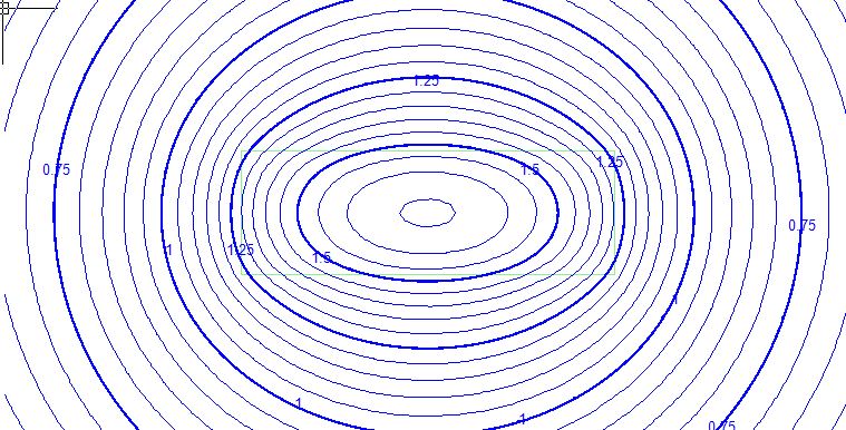
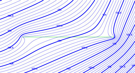
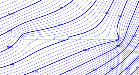
Check 12: Check of Anaqsim drain line boundary.
Checks drain line boundary, interdomain boundary. This compares two models with uniform recharge within a circular constant head boundary. The two models are identical, but one has a drain constructed with a line drain element and in the other, the drain is represented as a separate domain with finite width and the same equivalent conductivity as the line drain. The plots below are plots of heads near the drain in the two models and show nearly identical patterns. The files for the two models are DrainCheck1.anaq and DrainCheck2.anaq.
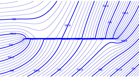
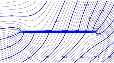
Check 13: Check of Anaqsim leaky barrier line boundary.
Checks leaky barrier line boundary, interdomain boundary. This compares two models with uniform recharge within a circular constant head boundary. The two models are identical, but one has a leaky barrier constructed with a leaky barrier line boundary and in the other, the leaky barrier is represented as a separate domain with finite width and the same equivalent resistance as the leaky barrier line boundary. The plots below are plots of heads near the barrier in the two models and show nearly identical patterns. The files for the two models are LeakyBarrierCheck1.anaq and LeakyBarrierCheck2.anaq.
Check 14: Uniform flow in a confined/unconfined aquifer with uniform recharge.
Checks confined/unconfined domain, constant head line boundary, normal flux line boundary, uniform recharge, 3D pathlines. This is the same as check2, but with a combined confined/unconfined domain. The domain goes from elevation 0 to 10. Head at the left is fixed at 15 (confined) and head at the right is fixed at 2 (unconfined). Flow over the entire model is from left to right. Over the 1000 unit distance from left to right, the uniform recharge adds an additional 0.50 to the domain discharge, which it does. The domain discharge (specific discharge times saturated thickness) is about 0.044 at the left edge and about 0.544 at the right edge. At the transition from confined to unconfined (h=10), the head, domain discharge, specific discharge, pathline elevation, and saturated thickness are all continuous as they should be. Within both the confined and unconfined portions of the model these variables are all properly related. Input file: check14.anaq
Check 15: Uniform flow in a two-layer confined/unconfined aquifer with uniform recharge.
Checks confined/unconfined domain, spatially-variable area sinks for vertical leakage, constant head line boundary, normal flux line boundary, uniform recharge, 3D pathlines, minimum saturated thickness where head drops to base of unconfined domain. This is the same as check14, but with two layers, both of which are combined confined/unconfined domains. The upper domain (level 1) spans elevation 5-10 and the lower domain (level 2) spans elevation 0-5. The vertical conductivity is high enough that there are very small head differences between the two levels, so the solution should be nearly identical to check 14, which it is. Heads in level 1 fall below the base (5) at the right side of the model, where the minimum saturated thickness (0.0001 * 5) is invoked; discharges in this zone are very small. The graph below shows aquifer discharge (Qx) as a function of x in each layer and the sum of the two. The sum is nearly identical to a similar plot for check 14, as expected. Input file: check15.anaq.

Check 16: Head-dependent normal flux (3rd type) boundary
- One model uses the head-dependent normal flux boundary at x = -500 with conductance C/b = 0.001 and h* = 15.0, (Check3rdType.anaq).
- The other model doesn’t have the 3rd type boundary, but instead has an equivalent finite width 2nd domain that extends from -600 < x < -500. The transmissivity (T) of this 2nd domain is 1/10th the T of the other domain. A head-specified boundary with h = 15.0 is at x = -600. The conductance of this 2nd domain is equivalent to the boundary conductance C/b = 0.1/100 = 0.001 in the other model (Check3rdType_alternate.anaq).
Both models result in h=13.50 and domain discharge Qx = -T (dh/dx) = 0.01500 at x=-500. See the contour plots compared below. Changing the model so that it is unconfined yields similar good comparisons between the model with the 3rd type boundary and the model with an equivalent finite 2nd domain (Check3rdType_unconfined.anaq, Check3rdType_unconfined_alternate.anaq).

Check 17: Check of vertical leakage over polygon tool
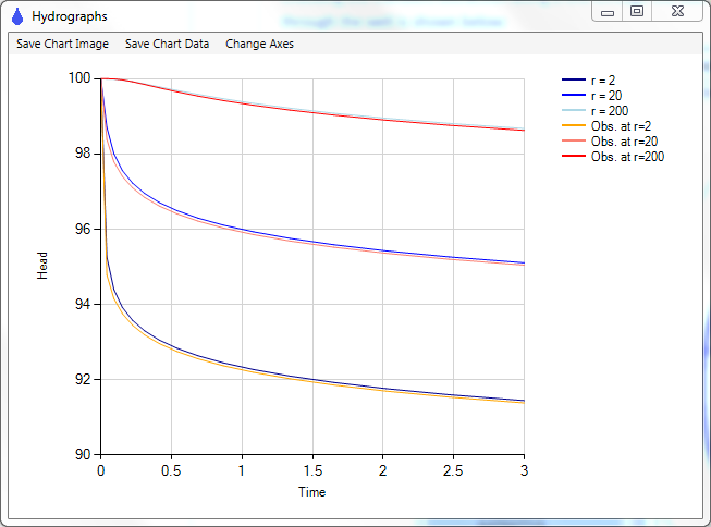
Check 18: Multi-layer pumping test comparison with MLU
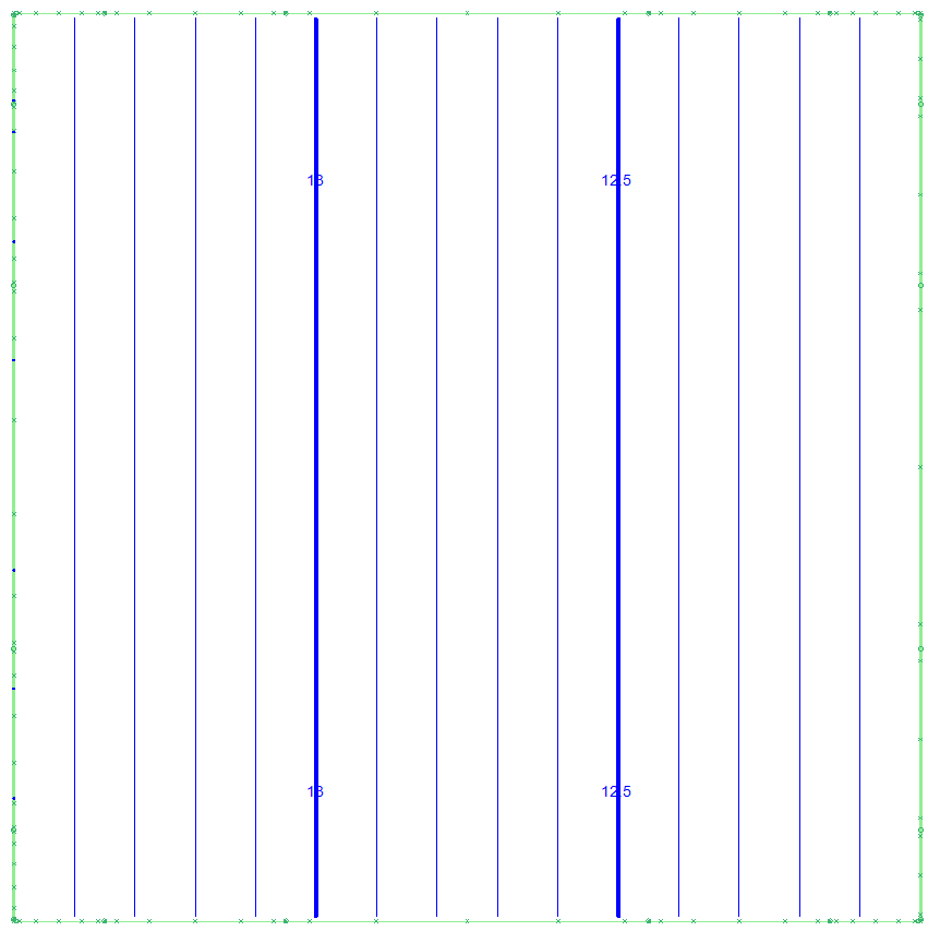
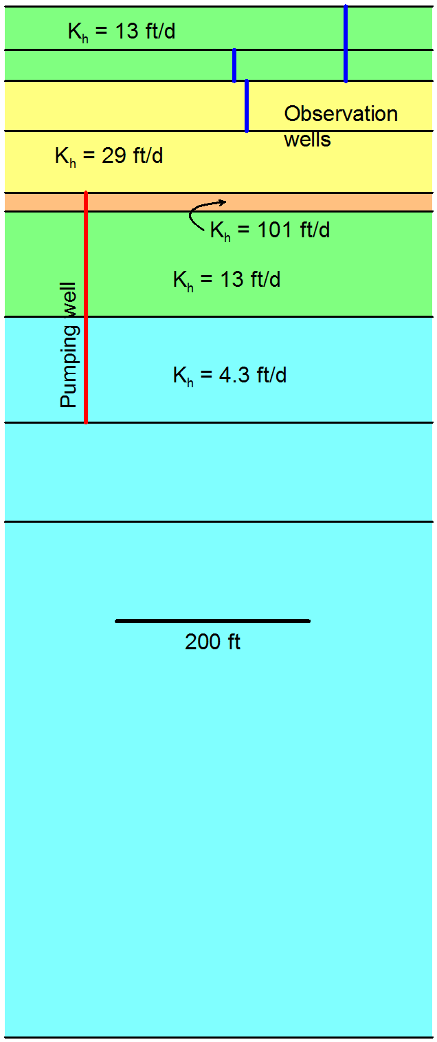 The models have 9 layers that are all confined and isotropic in the plane of the layering, as shown at left. The vertical hydraulic conductivity of each layer equals 1/5th the horizontal conductivity. The pumping well spans three of the 9 levels including the very transmissive 5th layer. Three shallow observation wells shown in the section were monitored in addition to the pumping well. The AnAqSim model uses a large number of time steps to minimize differences due to finite difference time stepping.
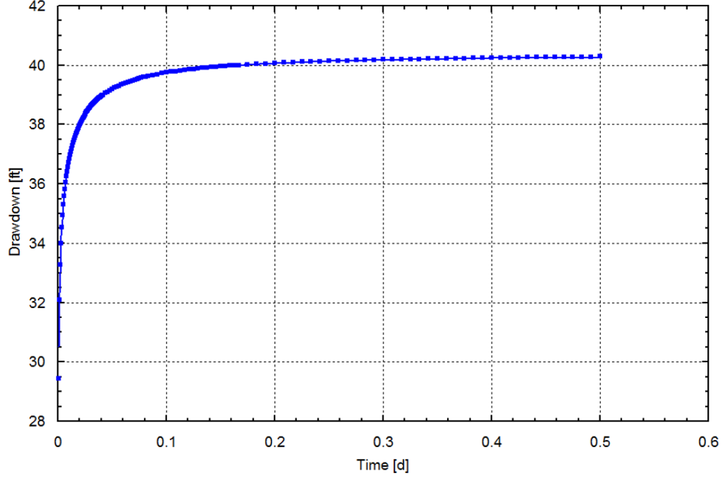
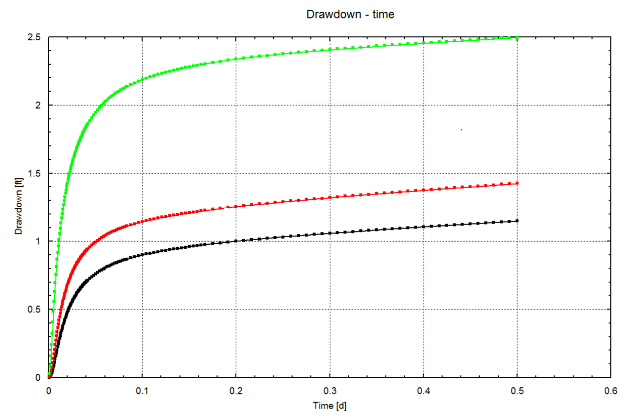
The model-simulated drawdowns in both the pumping well and in the three observation wells are essentially identical as the following plots show. AnAqSim simulation results are the lines and MLU simulation results are dots. (checkPumpingTestMLU.anaq)
Check 19: 3D pathline tracing comparison with Modflow
